Tips tutor truly working on science and technology in which there is included additional tools for educational purpose as well as daily life routine. we are deeply focusing on to provide you an effective and updated computer learning stuff through which you can make your work and educational life more easier today is the age of work from home so this is the exact reason we will providing you the best quality ideas to make money online from home through a lot of computer and mobile tools like MS
When you need an equation to reliably allude to a specific cell, regardless of whether you duplicate or move the recipe somewhere else on the worksheet, you have to utilize a flat out cell reference. A flat out cell reference is a cell address that contains a dollar sign ($) in the line or segment facilitate, or both. When you enter a cell reference in an equation, Excel expect it is a relative reference unless you change it to a flat out reference. In the event that you need some portion of a recipe to remain a relative reference, expel the dollar sign that shows up before the section letter or column number.
In case you're endeavoring to work out a normal, you're attempting to ascertain what the most widely
recognized esteem is. For instance, if a class of eight understudies took exams, you might need to recognize what the normal exam score was. As it were, what result most understudies can hope to get. Keeping in mind the end goal to ascertain a normal, you'd include each of the eight exam scores and partition by what number of understudies took the exam. So if the aggregate for each of the eight understudies was 400, separating by 8 would get you 50 as the normal review. In the event that any understudies were beneath the normal, you can tell initially.
In Excel , there is a simple approach to compute the normal of a few numbers - simply utilize the inbuilt Average capacity.
Begin another spreadsheet and enter the accompanying exams scores in cells A1 to A8,
be that as it may, shape this capacity you can without much of a stretch shield your Company and cash from big Loss just wach this video
The Excel CELING capacity restores a surrendered number adjusted to a predefined numerous. For instance, =CEILING(A1,5) could be utilized to cycle a cost in A1 to the closest 5 dollars. Roof dependably gathers together, far from zero.
Reason
Cycle a number up to the closest determined various
Return esteem
An adjusted number.
Linguistic structure
=CEILING (number, various)
Contentions
number - The number that ought to be adjusted.
various - The numerous to utilize when adjusting.
Use notes
Roof works like the MROUND work, yet CEILING dependably gathers together, far from zero.
Roof can be a can be a valuable capacity to set evaluating after cash change, rebates, and so on.
Roof equation cases
Exceed expectations equation: Round a number up to next half
Cycle a number up to next half
On the off chance that you have to cycle a number up to the following half, you can utilize the CEILING capacity, which dependably gathers together in view of a provided various. Note that MROUND likewise adjusts in light of a provided different, yet it generally adjusts...
Exceed expectations equation: Next semiweekly payday from date
Next every other week payday from date
Next every other week payday from dateTo get the following payday - accepting a semiweekly calendar, with paydays on Friday - you can utilize an equation in view of the CEILING capacity. In the case appeared, the recipe in C6 is: =CEILING(...
Exceed expectations recipe: Round a number up to closest numerous
Cycle a number up to closest various
In the event that you have to cycle a number up to the closest determined various (i.e. cycle a number up to the closest dollar, up to the closest $.25, up to the closest various of 5, and so forth.) you can utilize the CEILING capacity. In the...
Exceed expectations recipe: Round by package estimate
Round by package estimate
To round up to the following pack estimate, you can utilize the CEILING capacity which consequently gathers together far from zero. In the illustration appeared, we require a specific number of things, and the things come in particular package sizes....
Exceed expectations recipe: Round to closest 5
Round to closest 5
In the event that you have to cycle a number to the closest different of 5, you can utilize the MROUND capacity and supply 5 for number of digits. How this equation functions In the case, cell C6 contains this recipe: =MROUND(B6,5) The...
Exceed expectations recipe: Shade substituting gatherings of n lines
Shade rotating gatherings of n lines
To feature pushes in gatherings of "n" (i.e. shade each 3 pushes, each 5 lines, and so on.) you can apply contingent designing with a recipe in view of the ROW, CEILING and ISEVEN capacities. In the case appeared, the equation...
Watch this fpr understanding the method of ceiling formula
This Excel instructional exercise discloses how to utilize the Excel CELL work with language structure and cases.
Depiction
The Microsoft Excel CELL capacity can be utilized to recover data about a cell. This can incorporate substance, designing, estimate, and so on.
The CELL work is a worked in work in Excel that is classified as an Information Function. It can be utilized as a worksheet work (WS) in Excel. As a worksheet work, the CELL capacity can be entered as a component of a recipe in a cell of a worksheet.
Language structure
The language structure for the CELL work in Microsoft Excel is:
CELL( sort, [range] )
Parameters or Arguments
sort
The kind of data that you'd get a kick out of the chance to recover for the cell. sort can be one of the accompanying esteems:
ValueExplanation
"address"Address of the cell. On the off chance that the cell alludes to a range, it is the primary cell in the range.
"col"Column number of the cell.
"color"Returns 1 if the shading is a negative esteem; Otherwise it returns 0.
"contents"Contents of the upper-left cell.
"filename"Filename of the record that contains reference.
"format"Number configuration of the cell. See illustration arranges beneath.
"parentheses"Returns 1 if the cell is designed with enclosures; Otherwise, it returns 0.
"prefix"Label prefix for the cell.
* Returns a solitary quote (') if the cell is left-adjusted.
* Returns a twofold quote (") if the cell is correct adjusted.
* Returns a caret (^) if the cell is focus adjusted.
* Returns an oblique punctuation line (\) if the cell is fill-adjusted.
* Returns an unfilled content an incentive for all others.
"protect"Returns 1 if the cell is bolted. Returns 0 if the cell is not bolted.
"row"Row number of the cell.
"type"Returns "b" if the cell is void.
Returns "l" if the cell contains a content steady.
Returns "v" for all others.
"width"Column width of the cell, adjusted to the closest whole number.
"organize"
For the "organization" esteem, depicted over, the qualities returned are as per the following:
Returned Value
for "format"Explanation
"G"General
"F0"0
",0"#,##0
"F2"0.00
",2"#,##0.00
"C0"$#,##0_);($#,##0)
"C0-"$#,##0_);[Red]($#,##0)
"C2"$#,##0.00_);($#,##0.00)
"C2-"$#,##0.00_);[Red]($#,##0.00)
"P0"0%
"P2"0.00%
"S2"0.00E+00
"G"# ?/? or, then again # ??/??
"D4"m/d/yy or m/d/yy h:mm or mm/dd/yy
"D1"d-mmm-yy or dd-mmm-yy
"D2"d-mmm or dd-mmm
"D3"mmm-yy
"D5"mm/dd
"D6"h:mm:ss AM/PM
"D7"h:mm AM/PM
"D8"h:mm:ss
"D9"h:mm
extend
Discretionary. It is the cell (or range) that you wish to recover data for. On the off chance that the range parameter is overlooked, the CELL capacity will accept that you are recovering data for the last cell that was changed.
The Excel CHOOSE work restores an incentive from a rundown utilizing a given position or record. For instance, CHOOSE(2,"red","blue","green") returns "blue", since blue is the second esteem recorded after the list number. The qualities gave to CHOOSE can incorporate references.
Purpose
Get an incentive from a rundown in light of position
Return value
The incentive at the given position.
Syntax
=CHOOSE (index_num, value1, [value2], ...)
Contentions
index_num - The incentive to pick. A number in the vicinity of 1 and 254.
value1 - The primary incentive from which to pick.
value2 - [optional] The second an incentive from which to pick.
Use notes
Pick can deal with up to 254 esteems. Index_num returns an esteem in view of it's position in the rundown. For instance, if index_num is 2, value2 is returned.
Qualities can likewise be references. For instance, the address A1, or the reaches A1:10 or B2:B15 can be provided as qualities.
Example Of Choose Formua
Excel expectations CODE and CHAR Functions, VBA Asc and Chr Functions
Excel expectations Text and String Functions:
Excel expectations CODE and CHAR Functions, VBA Asc and Chr Functions, with cases.
1. Utilizing VBA Chr and Asc capacities to change over exceed expectations section number to comparing segment letter, and segment letter to segment number.
3. Exceed expectations Text and String Functions: TRIM and CLEAN.
4. Exceed expectations Text and String Functions: LEFT, RIGHT, MID, LEN, FIND, SEARCH, REPLACE, SUBSTITUTE.
Exceed expectations CODE Function (Worksheet)
The CODE Function restores the distinguishing numeric code of the principal character in a content string. A 'character set' maps characters to their distinguishing code esteems, and may change crosswise over working conditions viz. Windows, Macintosh, and so on. The Windows working condition utilizes the ANSI character set, while Macintosh utilizes the Macintosh character set. The returned numeric code relates to this character set - for a Windows PC, Excel utilizes the standard ANSI character set to restore the numeric code. Sentence structure: CODE(text_string). The text_string contention is the content string whose initially character's numeric code is returned.
What might as well be called exceed expectations CODE work in vba is the Asc work. Note that the Excel CODE work is the backwards of the Excel CHAR work. The equation =CODE(CHAR(65)) returns 65, on the grounds that =CHAR(65) restores the character "An" and =CODE("A") returns 65.
In a Windows PC, Code capacity will return esteems as takes after:
=CODE("A") returns 65.
=CODE("B") returns 66.
=CODE("a") returns 97.
=CODE("b") returns 98.
=CODE("0") returns 48.
=CODE("1") returns 49.
=CODE("- 1") returns 45, which is the code for "- " (hyphen) .
=CODE(" ") , take note of the space between altered commas, returns 32.
=CODE(""), no space between modified commas, restores the #VALUE! mistake esteem.
=CODE("America") returns 65, which is the code for "A", the principal character in the content string.
=CODE(A1) returns 66, utilizing cell reference. On the off chance that phone A1 contains the content "Bond", CODE(A1) returns 66, which is the code for "B", the main character in the content string.
=CODE("?") returns 63.
=CODE("™") returns 153.
Exceed expectations CHAR Function (Worksheet)
Utilize the CHAR Function to restore the character recognized to the predefined number. A 'character set' maps characters to their distinguishing code esteems, and may differ crosswise over working conditions viz. Windows, Macintosh, and so forth. The Windows working condition utilizes the ANSI character set, while Macintosh utilizes the Macintosh character set. The returned character compares to this character set - for a Windows PC, Excel utilizes the standard ANSI character set. Linguistic structure: CHAR(number). The number contention is a number in the vicinity of 1 and 255 which recognizes the returned character. The capacity restores the #VALUE! mistake esteem if this contention is not a number in the vicinity of 1 and 255.
What might as well be called exceed expectations CHAR work in vba is the Chr work. Note that the Excel CHAR work is the opposite of the Excel CODE work. The equation =CHAR(CODE("A")) restores An, on the grounds that =CODE("A") restores the number 65 and =CHAR(65) restores A.
In a Windows PC, Char capacity will return esteems as takes after:
=CHAR(65) restores the character "A".
=CHAR(37) restores the character "%".
=CHAR(260) restores the #VALUE! mistake esteem.
=CHAR(163) restores the character "£".
=CHAR(A1) restores the character "B", utilizing cell reference. On the off chance that cell A1 contains the number 66, CHAR(A1) restores the character "B".
Cases of utilizing the Excel CODE and CHAR Functions
Evolving case (capitalized/lowercase) of letters in order in a string
Equation =CHAR(CODE(A1)+32) restores the lowercase letter "b", if cell A1 contains the capitalized letter "B". This is on the grounds that in the ANSI character set, the lowercase letter sets show up after capitalized letters in order, in an alphabetic request, with a distinction of precisely 32 numbers. Likewise, =CHAR(CODE(A1)- 32) restores the capitalized letter "B", if cell A1 contains the lowercase letter "b".
Change over first character of the primary word in a content string (comprising of letters), to lowercase, and first character of every ensuing word to capitalized. To change over the string "we like james bond" in cell A1 to "we Like James Bond" utilize the accompanying recipe:
=PROPER(A1) restores the content string "We Like James Bond".
=CHAR(CODE(LEFT(PROPER(A1)))+32) restores the lowercase content "w".
The recipe replaces the principal character of the content, by first underwriting it and after that changing over it to lowercase utilizing CHAR/CODE capacities.
It might however be noticed, that the exceed expectations UPPER (or LOWER) capacity can likewise be utilized as interchange to CHAR/CODE capacities. For this situation the Formula =REPLACE(PROPER(A1),1,1,LOWER(LEFT(PROPER(A1)))) will likewise give a similar outcome and restore the string "we Like James Bond".
- - - - - - - - - -
Making the above equation more unpredictable:
Change over first character of the second word in a content string (comprising of letters) to lowercase, and the primary character of every other word to capitalized (wherein words are isolated by a solitary space). To change over the string "we Like James bond" in cell A1 to "We like James Bond" utilize the accompanying equation:
=CHAR(CODE(MID(PROPER(A1),FIND(" ",A1)+1,1))+32) restores the content "l".
- - - - - - - - - -
In the event that a content string has unpredictable dispersing (ie. having lead spaces and numerous spaces between words), embed the TRIM capacity which expels all spaces from content with the exception of single spaces between words:
Note: notwithstanding the CHAR, CODE, LEFT and MID capacities, we have additionally utilized the exceed expectations worksheet PROPER capacity. Linguistic structure: PROPER(text). This capacity: (I) Capitalizes any letter in a content string which takes after a non-letter character, and furthermore the primary letter of the content string; (ii) Converts to Lowercase every single other letter.
how to use convert formula in Excel part 1 On the off chance that you've ever need to make an interpretation of Celsius to Fahrenheit, miles to kilometers, or teaspoons to mugs, all you require is the helpful CONVERT work in Excel. Basically enter your esteem, its estimation unit, and the objective unit for change, and you'll find your solution. Here are some helpful cases: =CONVERT(30.4,"C","F") =CONVERT(65,"mi","km") =CONVERT(10,"tsp","cup") You don't have to remember the majority of the units that are accessible. Simply sort "=CONVERT(" trailed by the esteem. When you enter the comma to move to the units area of the capacity, you'll see a rundown of accessible units to browse in the equation bar: Select units for CONVERT work Utilize the scrollbar to discover your unit and either double tap or snap + TAB to choose it. At that point enter another comma after the unit's nearby quote to raise the rundown again to choose your objective unit, and afterward shut the enclosure and hit Enter. Simply make sure that the units you select for both are connected estimations or you'll get a blunder. You can't change over years to pounds, for example. Luckily, Excel as a rule compels the rundown of accessible measures to ones that match your beginning unit: Select target units Note that not every single accessible unit might be recorded. While changing over miles, I just discovered meters - however evolving the "m" to "km" brought about transformation to kilometers. Suzanne
Labels Excel capacities Office 2007 Office 2010 watch live how to do this
This article describes the formula syntax and usage of the CORREL function in Microsoft Excel.
Description
Returns the correlation coefficient of the Array1 and Array2 cell ranges. Use the correlation coefficient to determine the relationship between two properties. For example, you can examine the relationship between a location's average temperature and the use of air conditioners. Syntax
CORREL(array1, array2)
The CORREL function syntax has the following arguments:
Array1 Required. A cell range of values.
Array2 Required. A second cell range of values.
Remarks
If an array or reference argument contains text, logical values, or empty cells, those values are ignored; however, cells with the value zero are included.
If Array1 and Array2 have a different number of data points, CORREL returns the #N/A error value.
If either Array1 or Array2 is empty, or if s (the standard deviation) of their values equals zero, CORREL returns the #DIV/0! error value.
The equation for the correlation coefficient is:
Equation
where
x and y
are the sample means AVERAGE(array1) and AVERAGE(array2).
Example
Copy the example data in the following table, and paste it in cell A1 of a new Excel worksheet. For formulas to show results, select them, press F2, and then press Enter. If you need to, you can adjust the column widths to see all the data.
Data1
Data2
3
9
2
7
4
12
5
15
6
17
Formula
Description
Result
=CORREL(A2:A6,B2:B6)
Correlation coefficient of the two data sets in columns A and B.
Using a combination of Excel functions and the date of birth, you can easily calculate age in Excel. You can either calculate the age till the current date or between the specified period of time.
The technique shown here can also be used in other situations such as calculating the duration of a project or the tenure of the service.
How to Calculate Age in Excel
In this tutorial, you’ll learn how to calculate age in Excel in:
The number of years elapsed till the specified date.
The number of Years, Months, and Days elapsed till the specified date.
You can also download the Excel Age Calculator Template.
Calculate Age in Excel – Years Only
Suppose you have the date of birth in cell B1, and you want to calculate how many years have elapsed since that date, here is the formula that’ll give you the result:
=DATEDIF(B1,TODAY(),"Y")
How to Calculate Age in Excel - Datedif years
If you have the current date (or the end date) in a cell, you can use the reference instead of the TODAY function. For example, if you have the current date in cell B2, you can use the formula:
=DATEDIF(B1,B2,"Y")
Now, let’s see how the DATEDIF function works.
DATEDIF function is provided for the compatibility with Lotus 1-2-3. One of the things that you’ll notice when you use this function is that there is no IntelliSense available for this function. No tool tip appears when you use this function.
How to Calculate Age in Excel - Datedif
This means that while you can use this function is Excel, you need to know the syntax and how many arguments this function takes.
Overview of the Excel DATEDIF function
Syntax: =DATEDIF(start_date, end_date, unit)
Excel DATEDIF function takes 3 arguments:
start_date: It’s a date that represents the starting date value of the period. It can be entered as text strings in double quotes, as serial number, or as a result of some other function, such as DATE().
end_date: It’s a date that represents the end date value of the period. It can be entered as text strings in double quotes, as serial number, or as a result of some other function, such as DATE().
unit: This would determine what type of result you get from this function. There are six different output that you can get from the DATEDIF function, based on what unit you use. Here are the units that you can use:
“Y” – returns the number of completed years in the specified time period.
“M” – returns the number of completed months in the specified time period.
“D” – returns the number of completed days in the specified period.
“MD” – returns the number of days in the period, but doesn’t count the ones in the Years and Months that have been completed.
“YM” – returns the number of months in the period, but doesn’t count the ones in the years that have been completed.
“YD” – returns the number of days in the period, but doesn’t count the ones in the years that have been completed.
You can also use the YEARFRAC function to calculate the age in Excel (in years) in the specified date range.
Here is the formula:
=INT(YEARFRAC(B1,TODAY()))
How to Calculate Age in Excel - YEARFRAC years
The YEARFRAC function returns the number of years between the two specified dates and then the INT function returns only the integer part of the value.
NOTE: It’s a good practice to use the DATE function to get the date value. It avoids any erroneous results that may occur when entering the date as text or any other format (which is not an acceptable date format).
Calculate Age in Excel – Years, Months, & Days
Suppose you have the date of birth in cell A1, here are the formulas:
To get the year value:
=DATEDIF(B1,TODAY(),"Y")
How to Calculate Age in Excel - Datedif Year Value
To get the month value:
=DATEDIF(B1,TODAY(),"YM")
How to Calculate Age in Excel - Datedif Month Value
To get the day value:
=DATEDIF(B1,TODAY(),"MD")
How to Calculate Age in Excel - Datedif Day Value
Now that you know how to calculate the years, months and days, you can combine these three to get a text that says 26 Years, 2 Months, and 13 Days. Here is the formula that will get this done:
=DATEDIF(B1,TODAY(),"Y")&" Years "&DATEDIF(B1,TODAY(),"YM")&" Months "&DATEDIF(B1,TODAY(),"MD")&" Days"
How to Calculate Age in Excel - combined
Note that the TODAY function is volatile and its value would change every day whenever you open the workbook or there is a change in it. If you want to keep the result as is, convert the formula result to a static value.
Download the Excel Age Calculator Template
Download File
Excel Functions Used:
Here is a list of functions used in this tutorial:
DATEDIF() – This function calculates the number of days, months, and years between two specified dates.
TODAY() – It gives the current date value.
YEARFRAC() – It takes the start date and the end date and gives you the number of years that have passed between the two dates. For example, if someone’s date of birth is 01-01-1990, and the current date is 15-06-2016, the formula would return 26.455. Here the integer part represents the number of years completed, and the decimal part represents additional days that have passed after 26 years.
DATE() – It returns the date value when you specify the Year, Month, and Day value arguments.
INT() – This returns the integer part of a value.
Advance Work Of Excel course and Advance Excel in now presented Tittle
how to use datedif formula how to find over all years ,months and days of any person in Excel
Calculate the days, months or years between two dates. See how to use the undocumented Excel DATEDIF function. See how to:
1) Calculate the number of completed days between two dates d
2) Calculate the number of completed months between two dates m
3) Calculate the number of completed years between two dates y
4) Calculate the number of days after completed years yd
5) Calculate the number of months after completed years my
6) Calculate the number of months after completed years ym subscribe my channel
(You tube) https://www.youtube.com/channel/UCT19oGQ6i6kEp5sz9R4GWOA
(Google+)
https://plus.google.com/u/0/115433594671281035281
(Blogger)
http://advanceworkofexcel.blogspot.com/
(Twitter)
https://twitter.com/saddam_khan45
(Facebook Page)
https://www.facebook.com/Advance-Work-Of-Excel-453336005013724/
Using Excel's wildcard
At times, you could want to apply positive string matching or seek features — like search — without understanding exactly what you're looking for. As an example, you could need to look for a kingdom that starts offevolved with the phrase "New" — but suit against all viable outcomes, along with "New Hampshire", "big apple", and "New Jersey". To do this, you can use something called a "wildcard" person to tell Excel that you're looking for some thing, but you are no longer precisely certain what but.
Think of Excel's wildcard characters like the jokers in a deck of playing cards. They can tackle any fee they need to.
Right here's some extra statistics on how wildcards work:
The fundamental wildcard shape
There are two key styles of wildcards in Excel. Here's what they appear to be and how you use them.
Wildcardnamerationalization
?Question markTakes the region of a unmarried person. As an instance, "Tr?Y" suits with "Tray", "Troy", and "Trey", however no longer "Trolley"
*AsteriskCan take the place of any wide variety of characters. For instance, "Tr*y" matches with "Tray", "Troy", and "Trolley".
~TildaTells Excel that the following character need to be treated as a regular character and no longer a wildcard. As an example, "Tr~?Y" suits most effective with "Tr?Y", not "Tray" or "Troy".
In line with the chart above, use the query mark (?) while you need to accept only a single man or woman, and the asterisk (*) when you need to just accept multiple characters.
Create Worksheet in Excel 2013 Inserting New Worksheet three new clean sheets constantly open when you start Microsoft Excel. Beneath steps explain you how to create a new worksheet if you need to begin every other new worksheet while you're running on a worksheet, otherwise you closed an already opened worksheet and need to begin a brand new worksheet.
Step 1 − proper click on the Sheet name and select Insert option.
New Sheet Step 2 − Now you will see the Insert conversation with pick Worksheet option as decided on from the general tab. Click on the ok button.
Insert conversation Now you should have your clean sheet as proven beneath equipped to start typing your textual content.
Blank Sheet you could use a brief reduce to create a clean sheet every time. Attempt the usage of the Shift+F11 keys and you may see a new clean sheet just like the above sheet is opened.
in this lesson, we'll study the maximum fundamental way to go into information in an Excel worksheet - by way of typing. In destiny training, we're going to observe a number of shortcuts for coming into statistics faster.
To enter records in Excel, simply pick out a cellular and begin typing. You'll see the text seem each within the mobile and in the system bar above.
To tell Excel to accept the statistics you've typed, press input. The facts can be entered at once, and the cursor will flow down one mobile.
You may also press the tab key in place of the input key. If you press tab, the cursor will circulate one mobile to the proper as soon as the statistics has been entered.
When Excel sees which you are typing right into a listing, pressing enter on the stop of the row will move the cursor down one row and back to the first column.
At any time at the same time as you're typing you could press the get away key to cancel. This brings Excel returned to the state it changed into in before you commenced typing.
While you want to delete data that has already been entered, simply pick the cells, and press the delete key. you can also see this video to increase your input performance for more Tutorial to related Topics
Lesson 8 -How can save Excel Workbook_how to Save editing changes
Save your workbook
Applies To: Excel 2013 wherever you need to keep your workbook (for your pc or the internet, as an example), you do all of your saving on the file tab.
Whilst you’ll use keep or press Ctrl+S to keep an present workbook in its cutting-edge area, you want to apply keep As to save your workbook for the primary time, in a specific area, or to create a duplicate of your workbook in the equal or some other region. Here’s how:
click on report > store As.
Save As alternative at the report tab
under keep As, pick out the area wherein you need to shop your workbook. For instance, to shop in your desktop or in a folder on your laptop, click on computer.
Pick a location choice TIP: To store on your One Drive vicinity, click on One Drive, after which sign up (or sign in). To add your own locations in the cloud, like an Office 365 SharePoint or a One Drive location, click upload an area.
Click on Browse to discover the vicinity you want for your documents folder.
To pick some other vicinity to your pc, click on computer, after which choose the exact area in which you need to save your workbook.
Within the report name field, enter a call for a brand new workbook. Input a unique call if you’re growing a replica of an existing workbook.
To keep your workbook in a exclusive record layout (like .Xls or .Txt), inside the save as kind listing (under the file name container), select the format you need.
Click on keep.
Pin your favorite shop location
when you’re performed saving your workbook, you may “pin” the location you stored to. This maintains the area to be had so you can use it once more to shop some other workbook. If you tend to save matters to the identical folder or region loads, this could be a terrific time saver! You can pin as many places as you want.
Click on report > shop As.
Under store As, select the location where you last saved your workbook. For instance, if you last stored your workbook to the files folder on your computer, and you need to pin that location, click on laptop.
Underneath current folders at the right, point to the location you need to pin. A push pin picture Push pin button appears to the proper.
Use the rush pin icon to pin your favored shop region
click the photo to pin that folder. The photograph now shows as pinned Pinned push pin icon . On every occasion you keep a workbook, this vicinity will seem on the top of the listing below current folders.
TIP: To unpin a vicinity, simply click the pinned push pin photograph Pinned push pin icon again. Activate Auto Recovery
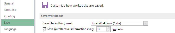
Excel automatically saves your workbook whilst you’re working on it, in case some thing happens, like the electricity going out. This is referred to as AutoRecovery. This isn’t similar to you saving your workbook, so don’t be tempted to depend upon AutoRecovery. Shop your workbook, regularly. However Autorecovery is a good manner to have a backup, simply in case some thing happens.
Ensure AutoRecovery is turned on:
click on document > options.
In the Excel alternatives conversation field, click store.
Keep choice in Excel alternatives
under save workbooks, make certain shop AutoRecover statistics every n mins is checked.
Set the minutes for a way regularly you want Excel to again up your paintings, and then click on ok.
if you want live guide line then see this
you can also learn From SID's Excel Expert Channel
Lesson 7 -what is the work of Page Layout menu In Excel_how can we use
Page Layout Tab in Microsoft Excel
Use web page format view to satisfactory-tune pages earlier than printing
Applies To: Excel 20013 earlier than you print a Microsoft office Excel worksheet that consists of a huge amount of records or more than one charts, you could quickly exceptional-tune it in the page format view to achieve professional-searching consequences. As in everyday view, you could trade the layout and format of facts, however further, you could use the rulers to measure the width and peak of the records, trade the page orientation, add or alternate web page headers and footers, set margins for printing, disguise or display gridlines, row and column headings, and specify scaling options. When you end running in page layout view, you could return to normal view.
Question will arise in your mind
What do you want to do? Use rulers in page format view trade web page orientation in page format view add or trade page headers and footers in page format view Set web page margins in page format view conceal or display headers, footers, and margins in page format view conceal or show gridlines, row headings, and column headings in web page layout view choose scaling alternatives in page layout view return to everyday view
Use rulers in page layout view
In web page format view, Excel affords a horizontal ruler and a vertical ruler so you can take specific measurements of cells, levels, objects, and web page margins. Rulers let you role items and to view or edit page margins directly on the worksheet.
Through default, the ruler shows the default devices which are distinct inside the local settings in control Panel, however you may alternate the devices to inches, centimeters, or millimeters. Rulers are displayed by default, but you could without difficulty cover them.
Alternate the measurement units
1:click the worksheet which you want to change in web page layout view.
2:On the View tab, inside the Workbook perspectives institution, click page layout View.
you can additionally click page format View Button on the repute bar.
3:Click the Microsoft office Button office button and then click on Excel options.
4:Inside the advanced class, underneath display, select the devices that you need to apply inside the Ruler gadgets list.
Hide or show the rulers
1:on the View tab, in the Workbook views organization, click page layout View.
you could additionally click web page layout View Button on the reputation bar.
2:On the View tab, in the show/hide organization, clean the Ruler test field to hide the rulers, or select the test box to show the rulers.
TIP: while the rulers are displayed, show Ruler is highlighted within the Sheet options organization.
Trade web page orientation in page layout view
1:click the worksheet that you need to alternate in web page format view.
2:At the View tab, inside the Workbook perspectives institution, click on page format View.
you can also click on page format View Button at the fame bar.
3:On the page format tab, within the page Setup organization, click Orientation, after which click Portrait or panorama.
Upload or exchange web page headers and footers in page layout view
1:click on the worksheet that you want to change in web page format view.
2:On the View tab, in the Workbook views group, click page format View.
you could also click on page layout View Button at the fame bar.
3:Do one of the following:
to feature a header or footer, point to click to feature header at the top of the worksheet web page or click on to feature footer at the bottom of the worksheet web page, after which click in the left, middle, or proper header or footer text box.
To change the textual content of a header or a footer, click the header or footer text box at the top or the bottom of the worksheet web page respectively, after which choose the textual content which you want to alternate.
TIP: you can additionally display headers or footers in regular view. At the Insert tab, inside the text group, click on Header & Footer. Excel displays page format view and positions the pointer in the header text box at the pinnacle of the worksheet page.
4:Type the brand new header or footer text.
NOTES:
to start a new line in a segment box, press input.
To delete a part of a header or footer, choose the element that you want to delete inside the section box, and then press DELETE or BACKSPACE. You could also click the text after which press BACKSPACE to delete the previous characters.
To consist of a single ampersand (&) within the text of a header or footer, use two ampersands. As an instance, to encompass "Subcontractors & services" in a header, type Subcontractors && offerings.
To shut the headers or footers, click everywhere within the worksheet, or press ESC.
Set web page margins in web page layout view
1:click on the worksheet which you want to alternate in web page layout view.
2:On the View tab, inside the Workbook perspectives group, click on web page layout View.
you may also click web page format View Button at the status bar.
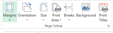
3:At the page format tab, inside the web page Setup group, click on Margins, and then click normal, slim, or wide.
For greater alternatives, click custom Margins, after which on the Margins tab, choose the margin sizes that you need.
4:To exchange margins with the aid of the usage of the mouse, do one of the following:
To trade the top or backside margin, click the pinnacle border or the lowest border of the margin vicinity inside the ruler. When a vertical double-headed arrow appears, drag the margin to the size that you need.
To exchange the proper or left margin, click the proper or left border of the margin place in the ruler. While a horizontal double-headed arrow seems, drag the margin to the size that you need.
A ScreenTip displays the margin size even as you're dragging the margin to the dimensions that you need.
The header and footer margins automatically modify whilst you change the page margins. You could also exchange the header and footer margins with the aid of using the mouse. Click on in the header or footer vicinity on the top or the lowest of the web page respectively, after which click on the ruler till the double-headed arrow appears. Drag the margin to the dimensions that you want.
Hide or display headers, footers, and margins in web page format view
Headers, footers, and margins are displayed via default in web page layout view. To cover them when you want greater workspace, do the subsequent:
1:click on the worksheet which you need to change in web page layout view.
2:On the View tab, inside the Workbook perspectives institution, click on web page layout View.
you can additionally click on web page format View Button on the fame bar.
3:Click on the brink of any border of the worksheet to cover or show the white space across the cells.
You may additionally click on among pages to hide or show the white area around the cells.
disguise or show gridlines, row headings, and column headings in page layout view
Gridlines, row headings, and column headings are displayed by means of default in web page layout view, but they're no longer printed automatically.
1:Click on the worksheet which you want to change in web page layout view.
2:At the View tab, within the Workbook perspectives organization, click web page format View.
you can additionally click on web page layout View Button at the status bar.
3:At the web page layout tab, inside the Sheet alternatives institution, do one or greater of the following:
to cover or show gridlines, below Gridlines, clean or choose the View check container.
To print gridlines, underneath Gridlines, pick the Print test field.
To cover or display row and column headings, under Headings, clean or pick out the View take a look at box.
To print row and column headings, under Headings, pick the Print take a look at container.
pick out scaling options in web page layout view
1:click the worksheet which you want to alternate in web page layout view.
2:At the View tab, in the Workbook perspectives institution, click on page layout View.
you may also click on page layout View Button at the popularity bar.
3:At the web page format tab, within the Scale to healthy group, do one of the following:
To lessen the width of the printed worksheet to fit a maximum quantity of pages, pick out the quantity of pages which you need within the Width listing.
To decrease the height of the printed worksheet to in shape a maximum number of pages, pick out the variety of pages which you need within the top list.
To increase or lower the broadcast worksheet to a percentage of its actual size, pick the proportion that you want in the Scale field.
observe: To scale a published worksheet to a percent of its actual length, the most width and top should be set to computerized.
Return to normal view
on the View tab, inside the Workbook perspectives institution, click ordinary.
you may additionally click ordinary Button at the popularity bar. you can also guide your self from video
you can also learn From SID's Excel Expert Channel
Lesson 6 -what is the work of Insert menu In Excel_how can we use
Insert Tab in Microsoft Excel
What's Insert tab and its makes use of?
We use Insert tab to insert the image, charts, filter out, hyperlink and many others. We use this option to insert the gadgets in Excel. To open the insert tab, press shortcut keys Alt+N.
below the Insert tab, we have 10 organizations:-
a) Tables: - We use this feature to insert the dynamic table, Pivot table and encouraged desk. Pivot table is used to create the precis of file with the built-in calculation, and we've choice to make our own calculation. Tables make it smooth to sort, filter and format the information within a sheet. This selection is likewise having advocated table which means on the idea of records, we can simply insert the table as consistent with the Excel’s advice.
b) instance: - We use this option to insert the photographs, on-line photos, Shapes, SmartArt and Screenshot. It method if we need to insert any image, we are able to use instance characteristic.
c) Apps: - We use this feature to insert an app into the file and, a good way to beautify the functionality, we will use web alternative.
Photo five
d) Charts: -Charts is very critical and beneficial function in Excel. In excel, we have extraordinary and exact numbers of readymade chart options. We've eight kinds of extraordinary charts in Excel:- Column, Bar, Radar, Line, region, combo, Pie and Bubbles chart. We can insert Pivot chart as well as advocated chart, and if we don’t recognise which chart we need to insert for the facts, we will use this selection to fulfil the requirement.
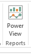
e) reports: -We use this selection to create a better file on the idea of the decisions we take for commercial enterprise. It makes the file more interactive and decipherable.
f) Sparklines: -Sparkline is a totally problematic and beneficial option introduced by using Microsoft Excel. On the premise of a selection, it could visualize the developments in a unmarried mobile as charts. We've 3 distinct kinds of cellular charts:- Line, Column and Win/Loss chart.
g) Filters: -We use this feature to clear out records visually and filter out dates interactively. We have 2 options: Slicers and Timeline. We use Slicer to make the short and easier to filter out tables, Pivot tables, Pivot Charts and cube features. Timeline makes it faster and easier to choose time durations with the intention to filter out Pivot Tables, Pivot Charts and dice feature.
h) hyperlinks: -
We use this option to create the hyperlink within the record for the fast get right of entry to to webpage and files. We can also use it to get entry to one-of-a-kind locations within the record. Image 10
i) text: -We use this option to insert the textual content box, Header and Footer, phrase art, Signature and items. We insert textual content field to jot down something inside the photo layout. We use Header and Footer alternatives to place the content at the top and backside of the web page. Phrase art makes the text fashionable. Insert the upload Signature strains that designate the man or woman who is meant to sign it. And item alternative works for embedded items, like documents or other documents we've inserted into the record
j) Symbols: - We use this feature to insert the symbols and equation. Equation is used to insert the commonplace mathematical equations for your report and also we are able to add equation through the use of the mathematical symbols. We use Symbols to insert the symbols which are not on the keyboard and, to create the equation, we use the symbols from right here.
for live guidance
you can also learn From SID's Excel Expert Channel