Tips tutor truly working on science and technology in which there is included additional tools for educational purpose as well as daily life routine. we are deeply focusing on to provide you an effective and updated computer learning stuff through which you can make your work and educational life more easier today is the age of work from home so this is the exact reason we will providing you the best quality ideas to make money online from home through a lot of computer and mobile tools like MS
This article describes the formula syntax and usage of the CORREL function in Microsoft Excel.
Description
Returns the correlation coefficient of the Array1 and Array2 cell ranges. Use the correlation coefficient to determine the relationship between two properties. For example, you can examine the relationship between a location's average temperature and the use of air conditioners. Syntax
CORREL(array1, array2)
The CORREL function syntax has the following arguments:
Array1 Required. A cell range of values.
Array2 Required. A second cell range of values.
Remarks
If an array or reference argument contains text, logical values, or empty cells, those values are ignored; however, cells with the value zero are included.
If Array1 and Array2 have a different number of data points, CORREL returns the #N/A error value.
If either Array1 or Array2 is empty, or if s (the standard deviation) of their values equals zero, CORREL returns the #DIV/0! error value.
The equation for the correlation coefficient is:
Equation
where
x and y
are the sample means AVERAGE(array1) and AVERAGE(array2).
Example
Copy the example data in the following table, and paste it in cell A1 of a new Excel worksheet. For formulas to show results, select them, press F2, and then press Enter. If you need to, you can adjust the column widths to see all the data.
Data1
Data2
3
9
2
7
4
12
5
15
6
17
Formula
Description
Result
=CORREL(A2:A6,B2:B6)
Correlation coefficient of the two data sets in columns A and B.
Using a combination of Excel functions and the date of birth, you can easily calculate age in Excel. You can either calculate the age till the current date or between the specified period of time.
The technique shown here can also be used in other situations such as calculating the duration of a project or the tenure of the service.
How to Calculate Age in Excel
In this tutorial, you’ll learn how to calculate age in Excel in:
The number of years elapsed till the specified date.
The number of Years, Months, and Days elapsed till the specified date.
You can also download the Excel Age Calculator Template.
Calculate Age in Excel – Years Only
Suppose you have the date of birth in cell B1, and you want to calculate how many years have elapsed since that date, here is the formula that’ll give you the result:
=DATEDIF(B1,TODAY(),"Y")
How to Calculate Age in Excel - Datedif years
If you have the current date (or the end date) in a cell, you can use the reference instead of the TODAY function. For example, if you have the current date in cell B2, you can use the formula:
=DATEDIF(B1,B2,"Y")
Now, let’s see how the DATEDIF function works.
DATEDIF function is provided for the compatibility with Lotus 1-2-3. One of the things that you’ll notice when you use this function is that there is no IntelliSense available for this function. No tool tip appears when you use this function.
How to Calculate Age in Excel - Datedif
This means that while you can use this function is Excel, you need to know the syntax and how many arguments this function takes.
Overview of the Excel DATEDIF function
Syntax: =DATEDIF(start_date, end_date, unit)
Excel DATEDIF function takes 3 arguments:
start_date: It’s a date that represents the starting date value of the period. It can be entered as text strings in double quotes, as serial number, or as a result of some other function, such as DATE().
end_date: It’s a date that represents the end date value of the period. It can be entered as text strings in double quotes, as serial number, or as a result of some other function, such as DATE().
unit: This would determine what type of result you get from this function. There are six different output that you can get from the DATEDIF function, based on what unit you use. Here are the units that you can use:
“Y” – returns the number of completed years in the specified time period.
“M” – returns the number of completed months in the specified time period.
“D” – returns the number of completed days in the specified period.
“MD” – returns the number of days in the period, but doesn’t count the ones in the Years and Months that have been completed.
“YM” – returns the number of months in the period, but doesn’t count the ones in the years that have been completed.
“YD” – returns the number of days in the period, but doesn’t count the ones in the years that have been completed.
You can also use the YEARFRAC function to calculate the age in Excel (in years) in the specified date range.
Here is the formula:
=INT(YEARFRAC(B1,TODAY()))
How to Calculate Age in Excel - YEARFRAC years
The YEARFRAC function returns the number of years between the two specified dates and then the INT function returns only the integer part of the value.
NOTE: It’s a good practice to use the DATE function to get the date value. It avoids any erroneous results that may occur when entering the date as text or any other format (which is not an acceptable date format).
Calculate Age in Excel – Years, Months, & Days
Suppose you have the date of birth in cell A1, here are the formulas:
To get the year value:
=DATEDIF(B1,TODAY(),"Y")
How to Calculate Age in Excel - Datedif Year Value
To get the month value:
=DATEDIF(B1,TODAY(),"YM")
How to Calculate Age in Excel - Datedif Month Value
To get the day value:
=DATEDIF(B1,TODAY(),"MD")
How to Calculate Age in Excel - Datedif Day Value
Now that you know how to calculate the years, months and days, you can combine these three to get a text that says 26 Years, 2 Months, and 13 Days. Here is the formula that will get this done:
=DATEDIF(B1,TODAY(),"Y")&" Years "&DATEDIF(B1,TODAY(),"YM")&" Months "&DATEDIF(B1,TODAY(),"MD")&" Days"
How to Calculate Age in Excel - combined
Note that the TODAY function is volatile and its value would change every day whenever you open the workbook or there is a change in it. If you want to keep the result as is, convert the formula result to a static value.
Download the Excel Age Calculator Template
Download File
Excel Functions Used:
Here is a list of functions used in this tutorial:
DATEDIF() – This function calculates the number of days, months, and years between two specified dates.
TODAY() – It gives the current date value.
YEARFRAC() – It takes the start date and the end date and gives you the number of years that have passed between the two dates. For example, if someone’s date of birth is 01-01-1990, and the current date is 15-06-2016, the formula would return 26.455. Here the integer part represents the number of years completed, and the decimal part represents additional days that have passed after 26 years.
DATE() – It returns the date value when you specify the Year, Month, and Day value arguments.
INT() – This returns the integer part of a value.
Advance Work Of Excel course and Advance Excel in now presented Tittle
how to use datedif formula how to find over all years ,months and days of any person in Excel
Calculate the days, months or years between two dates. See how to use the undocumented Excel DATEDIF function. See how to:
1) Calculate the number of completed days between two dates d
2) Calculate the number of completed months between two dates m
3) Calculate the number of completed years between two dates y
4) Calculate the number of days after completed years yd
5) Calculate the number of months after completed years my
6) Calculate the number of months after completed years ym subscribe my channel
(You tube) https://www.youtube.com/channel/UCT19oGQ6i6kEp5sz9R4GWOA
(Google+)
https://plus.google.com/u/0/115433594671281035281
(Blogger)
http://advanceworkofexcel.blogspot.com/
(Twitter)
https://twitter.com/saddam_khan45
(Facebook Page)
https://www.facebook.com/Advance-Work-Of-Excel-453336005013724/
Create Worksheet in Excel 2013 Inserting New Worksheet three new clean sheets constantly open when you start Microsoft Excel. Beneath steps explain you how to create a new worksheet if you need to begin every other new worksheet while you're running on a worksheet, otherwise you closed an already opened worksheet and need to begin a brand new worksheet.
Step 1 − proper click on the Sheet name and select Insert option.
New Sheet Step 2 − Now you will see the Insert conversation with pick Worksheet option as decided on from the general tab. Click on the ok button.
Insert conversation Now you should have your clean sheet as proven beneath equipped to start typing your textual content.
Blank Sheet you could use a brief reduce to create a clean sheet every time. Attempt the usage of the Shift+F11 keys and you may see a new clean sheet just like the above sheet is opened.
Lesson 7 -what is the work of Page Layout menu In Excel_how can we use
Page Layout Tab in Microsoft Excel
Use web page format view to satisfactory-tune pages earlier than printing
Applies To: Excel 20013 earlier than you print a Microsoft office Excel worksheet that consists of a huge amount of records or more than one charts, you could quickly exceptional-tune it in the page format view to achieve professional-searching consequences. As in everyday view, you could trade the layout and format of facts, however further, you could use the rulers to measure the width and peak of the records, trade the page orientation, add or alternate web page headers and footers, set margins for printing, disguise or display gridlines, row and column headings, and specify scaling options. When you end running in page layout view, you could return to normal view.
Question will arise in your mind
What do you want to do? Use rulers in page format view trade web page orientation in page format view add or trade page headers and footers in page format view Set web page margins in page format view conceal or display headers, footers, and margins in page format view conceal or show gridlines, row headings, and column headings in web page layout view choose scaling alternatives in page layout view return to everyday view
Use rulers in page layout view
In web page format view, Excel affords a horizontal ruler and a vertical ruler so you can take specific measurements of cells, levels, objects, and web page margins. Rulers let you role items and to view or edit page margins directly on the worksheet.
Through default, the ruler shows the default devices which are distinct inside the local settings in control Panel, however you may alternate the devices to inches, centimeters, or millimeters. Rulers are displayed by default, but you could without difficulty cover them.
Alternate the measurement units
1:click the worksheet which you want to change in web page layout view.
2:On the View tab, inside the Workbook perspectives institution, click page layout View.
you can additionally click page format View Button on the repute bar.
3:Click the Microsoft office Button office button and then click on Excel options.
4:Inside the advanced class, underneath display, select the devices that you need to apply inside the Ruler gadgets list.
Hide or show the rulers
1:on the View tab, in the Workbook views organization, click page layout View.
you could additionally click web page layout View Button on the reputation bar.
2:On the View tab, in the show/hide organization, clean the Ruler test field to hide the rulers, or select the test box to show the rulers.
TIP: while the rulers are displayed, show Ruler is highlighted within the Sheet options organization.
Trade web page orientation in page layout view
1:click the worksheet that you need to alternate in web page format view.
2:At the View tab, inside the Workbook perspectives institution, click on page format View.
you can also click on page format View Button at the fame bar.
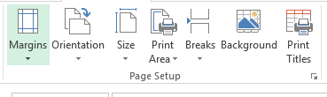
3:On the page format tab, within the page Setup organization, click Orientation, after which click Portrait or panorama.
Upload or exchange web page headers and footers in page layout view
1:click on the worksheet that you want to change in web page format view.
2:On the View tab, in the Workbook views group, click page format View.
you could also click on page layout View Button at the fame bar.
3:Do one of the following:
to feature a header or footer, point to click to feature header at the top of the worksheet web page or click on to feature footer at the bottom of the worksheet web page, after which click in the left, middle, or proper header or footer text box.
To change the textual content of a header or a footer, click the header or footer text box at the top or the bottom of the worksheet web page respectively, after which choose the textual content which you want to alternate.
TIP: you can additionally display headers or footers in regular view. At the Insert tab, inside the text group, click on Header & Footer. Excel displays page format view and positions the pointer in the header text box at the pinnacle of the worksheet page.
4:Type the brand new header or footer text.
NOTES:
to start a new line in a segment box, press input.
To delete a part of a header or footer, choose the element that you want to delete inside the section box, and then press DELETE or BACKSPACE. You could also click the text after which press BACKSPACE to delete the previous characters.
To consist of a single ampersand (&) within the text of a header or footer, use two ampersands. As an instance, to encompass "Subcontractors & services" in a header, type Subcontractors && offerings.
To shut the headers or footers, click everywhere within the worksheet, or press ESC.
Set web page margins in web page layout view
1:click on the worksheet which you want to alternate in web page layout view.
2:On the View tab, inside the Workbook perspectives group, click on web page layout View.
you may also click web page format View Button at the status bar.
3:At the page format tab, inside the web page Setup group, click on Margins, and then click normal, slim, or wide.
For greater alternatives, click custom Margins, after which on the Margins tab, choose the margin sizes that you need.
4:To exchange margins with the aid of the usage of the mouse, do one of the following:
To trade the top or backside margin, click the pinnacle border or the lowest border of the margin vicinity inside the ruler. When a vertical double-headed arrow appears, drag the margin to the size that you need.
To exchange the proper or left margin, click the proper or left border of the margin place in the ruler. While a horizontal double-headed arrow seems, drag the margin to the size that you need.
A ScreenTip displays the margin size even as you're dragging the margin to the dimensions that you need.
The header and footer margins automatically modify whilst you change the page margins. You could also exchange the header and footer margins with the aid of using the mouse. Click on in the header or footer vicinity on the top or the lowest of the web page respectively, after which click on the ruler till the double-headed arrow appears. Drag the margin to the dimensions that you want.
Hide or display headers, footers, and margins in web page format view
Headers, footers, and margins are displayed via default in web page layout view. To cover them when you want greater workspace, do the subsequent:
1:click on the worksheet which you need to change in web page layout view.
2:On the View tab, inside the Workbook perspectives institution, click on web page layout View.
you can additionally click on web page format View Button on the fame bar.
3:Click on the brink of any border of the worksheet to cover or show the white space across the cells.
You may additionally click on among pages to hide or show the white area around the cells.
disguise or show gridlines, row headings, and column headings in page layout view
Gridlines, row headings, and column headings are displayed by means of default in web page layout view, but they're no longer printed automatically.
1:Click on the worksheet which you want to change in web page layout view.
2:At the View tab, within the Workbook perspectives organization, click web page format View.
you can additionally click on web page layout View Button at the status bar.
3:At the web page layout tab, inside the Sheet alternatives institution, do one or greater of the following:
to cover or show gridlines, below Gridlines, clean or choose the View check container.
To print gridlines, underneath Gridlines, pick the Print test field.
To cover or display row and column headings, under Headings, clean or pick out the View take a look at box.
To print row and column headings, under Headings, pick the Print take a look at container.
pick out scaling options in web page layout view
1:click the worksheet which you want to alternate in web page layout view.
2:At the View tab, in the Workbook perspectives institution, click on page layout View.
you may also click on page layout View Button at the popularity bar.
3:At the web page format tab, within the Scale to healthy group, do one of the following:
To lessen the width of the printed worksheet to fit a maximum quantity of pages, pick out the quantity of pages which you need within the Width listing.
To decrease the height of the printed worksheet to in shape a maximum number of pages, pick out the variety of pages which you need within the top list.
To increase or lower the broadcast worksheet to a percentage of its actual size, pick the proportion that you want in the Scale field.
observe: To scale a published worksheet to a percent of its actual length, the most width and top should be set to computerized.
Return to normal view
on the View tab, inside the Workbook perspectives institution, click ordinary.
you may additionally click ordinary Button at the popularity bar. you can also guide your self from video
you can also learn From SID's Excel Expert Channel
Lesson 6 -what is the work of Insert menu In Excel_how can we use
Insert Tab in Microsoft Excel
What's Insert tab and its makes use of?
We use Insert tab to insert the image, charts, filter out, hyperlink and many others. We use this option to insert the gadgets in Excel. To open the insert tab, press shortcut keys Alt+N.
below the Insert tab, we have 10 organizations:-
a) Tables: - We use this feature to insert the dynamic table, Pivot table and encouraged desk. Pivot table is used to create the precis of file with the built-in calculation, and we've choice to make our own calculation. Tables make it smooth to sort, filter and format the information within a sheet. This selection is likewise having advocated table which means on the idea of records, we can simply insert the table as consistent with the Excel’s advice.
b) instance: - We use this option to insert the photographs, on-line photos, Shapes, SmartArt and Screenshot. It method if we need to insert any image, we are able to use instance characteristic.
c) Apps: - We use this feature to insert an app into the file and, a good way to beautify the functionality, we will use web alternative.
Photo five
d) Charts: -Charts is very critical and beneficial function in Excel. In excel, we have extraordinary and exact numbers of readymade chart options. We've eight kinds of extraordinary charts in Excel:- Column, Bar, Radar, Line, region, combo, Pie and Bubbles chart. We can insert Pivot chart as well as advocated chart, and if we don’t recognise which chart we need to insert for the facts, we will use this selection to fulfil the requirement.
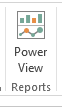
e) reports: -We use this selection to create a better file on the idea of the decisions we take for commercial enterprise. It makes the file more interactive and decipherable.
f) Sparklines: -Sparkline is a totally problematic and beneficial option introduced by using Microsoft Excel. On the premise of a selection, it could visualize the developments in a unmarried mobile as charts. We've 3 distinct kinds of cellular charts:- Line, Column and Win/Loss chart.
g) Filters: -We use this feature to clear out records visually and filter out dates interactively. We have 2 options: Slicers and Timeline. We use Slicer to make the short and easier to filter out tables, Pivot tables, Pivot Charts and cube features. Timeline makes it faster and easier to choose time durations with the intention to filter out Pivot Tables, Pivot Charts and dice feature.
h) hyperlinks: -
We use this option to create the hyperlink within the record for the fast get right of entry to to webpage and files. We can also use it to get entry to one-of-a-kind locations within the record. Image 10
i) text: -We use this option to insert the textual content box, Header and Footer, phrase art, Signature and items. We insert textual content field to jot down something inside the photo layout. We use Header and Footer alternatives to place the content at the top and backside of the web page. Phrase art makes the text fashionable. Insert the upload Signature strains that designate the man or woman who is meant to sign it. And item alternative works for embedded items, like documents or other documents we've inserted into the record
j) Symbols: - We use this feature to insert the symbols and equation. Equation is used to insert the commonplace mathematical equations for your report and also we are able to add equation through the use of the mathematical symbols. We use Symbols to insert the symbols which are not on the keyboard and, to create the equation, we use the symbols from right here.
for live guidance
you can also learn From SID's Excel Expert Channel
Lesson 5 -what is the work of Home menu In Excel_how can we use
Home Tab in Microsoft Excel
What is home tab and its uses? Domestic tab includes the maximum regularly used options which includes cut-copy-paste, font formatting, alignment, range, Conditional formatting, and so forth. All of the options are used to format the facts.
Photo 1
beneath the home tab, we've 7 agencies:-
photo 2
a) Clipboard: – This group includes regularly used instructions: reduce, replica, Paste and layout painter. Clipboard choice permits us to acquire textual content and photo objects and paste it.
Picture three
b) Font: – We use this feature to alternate the font fashion and font-size. We are able to make it formidable, italic and underline. Also, this institution consists of border patterns, fill shade, font shade.
Photo 4
c) Alignment: – We use this selection to trade the alignment of cell’s text to the right, left and center. Also, we can issue the text to pinnacle, backside, and center alignment. On this institution, we've Wrap text option to adjust and make the text seen inside a cell, and we can also merge 2 or extra cells, the use of merge option.
Photograph 5
d) wide variety: – We use this option to change the number formatting into popular, percentage, currency, Date, Time, Fraction and many others. We are able to boom and reduce the decimal and convert the number into accounting quantity.
Image 6
e) patterns: – In this selection, we've got Conditional Formatting, layout as table and cellular styles. Conditional formatting is used to spotlight the mobile or variety on the idea of situations. Format as table is having readymade desk format and mobile styles function extraordinary types of built-in patterns which can be a combination of Font fashion, Font color and Fill colour.
Photograph 7
f) Cells: – We use this feature to insert or delete cells, rows, columns and sheets. Additionally, we've got layout option to alter the peak, width of cells or variety. Using this option, we can cover or unhide the range, protect the workbook, rename the sheet call, fill the tab color, move or replica to sheets, lock the cells.
Image 8
g) modifying: – this option has auto Sum feature to go back the full of numbers and pass the textual content to proper, left, up and down, clean the format, content, comments and hyperlink; kind the information and locate and select option.
Photo 9
for live guidance
you can also learn From SID's Excel Expert Channel
Lesson 4 -Information about Record(File) Tab In Microsoft Excel
What is Record(File tab) and its uses?
Record tab consists of the fundamental required options together with New, Open, save, save as, Print, share, Export, and near alternatives. Other than the aforementioned options, we are able to locate account and Excel alternatives tab, too.
Picture 1
picture 2
a) data: - With this option, we are able to get the information about the precise Excel report. Created date, remaining modified date, writer call, homes, variations and so on.
Picture 3
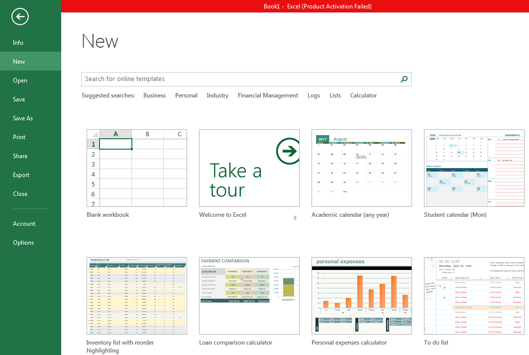
b) New: – We use this selection to open the brand new Excel record. We will open new document the usage of shortcut key, Ctrl+N or by Clicking on report tab > New > clean workbook. If Excel document isn't opened, then Press Window+R and type Excel, New Excel report will open.
Picture 4
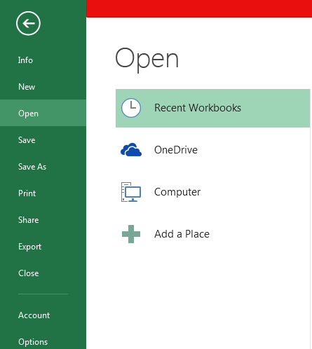
c) Open: – We use this feature to open the prevailing report (shortcut Ctrl+O). “Open” alternative appears and you may select to open the record.
Rather, file tab > Open > choose the document
Picture 5
d) keep: – We use this option to keep the cutting-edge document.
Shortcut: – Ctrl+S
route: – click on record tab >keep
e) store as: – We use this selection to make every other copy or keep the document at every other area. F12 is the shortcut key to save as the file or we are able to keep the record following those steps: – click on document tab > save as after which pick out the area.
Picture 6
f) Print: – We use this option to print the contemporary document. Ctrl+P is the shortcut key to print, or we can comply with those steps: – document > Print after which we will have the page setup option. We will set the page in step with our necessities.
Picture 7
g) percentage: – We use this option to share the file with a couple of users and send it over electronic mail. To share the report we will comply with the stairs: – click on on document tab >proportion.
Picture 8
h) Export: – We use this feature to export the report in PDF or XPS record and we can trade the report type as properly. To Export the document, we will observe the stairs: – click on file tab >Export. And then we can export it as in step with our requirement.
Picture 9
i) close: – We use this selection to close the document. Ctrl+W is the shortcut key to shut the workbook or we are able to comply with the stairs: – click on record tab >near, active report might be closed. Whilst we close the record, we get the confirmation message to store the file or not or cancel the command.
Picture 10
j) Account: – We use this selection to sign in to our office account and we will exchange office subject, too. We can follow the steps: – click on report tab >active, lively window will appear.
Picture 11
ok) options: – It turned into in the device menu of the preceding variations of 2007 MS. We use this feature to feature extra and superior capabilities, like Developer tab, power pivot, evaluation toolpak and lots of greater. Also, we can alternate default settings, like font size, font style, range of sheets etc. In Excel alternatives, we have 10 classes:-
1) wellknown
2) formulation
3) Proofing
4) keep
five) Language
6) superior
7) customise Ribbon
8) brief get entry to toolbar
9) upload Ins
10) accept as true with middle
picture 12
For live guidance
you can also learn From SID's Excel Expert Channel